The data pipeline of an inclinometer, stage by stage

An inclinometer measures rotation along two axes of inclination (φ and θ). Some sensors, such as the Move Solutions tiltmeter, incorporate a triaxial accelerometer that also adds vibrational acceleration values to the record. The final figure — say "0.42 mm of drift" — is the result of a chain of transformations applied to two raw numbers: the angle on the X axis and the angle on the Y axis.

What actually comes out of an inclinometer

At each sampling instant, an inclinometer returns a minimal record: angle X, angle Y, internal package temperature and UTC timestamp. Angles may arrive in degrees, millidegrees or microradians depending on the firmware.

For the TLT-STD-LR-2 inclinometer, repeatability is ±0.0008° (≈ 14 µrad) and accuracy is ±0.002° within the ±0.5° range. Exact figures should always be verified against the datasheet of the sensor actually installed.

From angle to displacement

The conversion from angle to linear displacement is geometric (and not static). If the sensor is mounted at distance L from the point of interest and rotates by a small angle θ, the displacement of that point relative to its initial position is:

Δx = L · sin(θ) ≈ L · θ (with θ in radians)

Here is an example. A bridge pier 12 m tall, sensor mounted at the top, measured rotation 0.002° — roughly 35 µrad. The horizontal displacement of the top relative to the base is 12 × 35 × 10⁻⁶ ≈ 0.42 mm.

"L" is the actual mechanical lever arm of the deformation mechanism. If the pier rotates around a plastic hinge formed 4 m from the base, the arm is 8 m. Getting the arm wrong introduces a multiplicative factor. An assumed arm of 12 m instead of 8 inflates the displacement by 50 %. No downstream filter will correct that error: L is a multiplicative factor that scales every reading proportionally. If the arm is overestimated by 50 %, every calculated displacement will be overestimated by 50 %, regardless of how many filters are applied before or after.

The choice of L is a structural-model engineering decision and must be documented in the monitoring plan with the same care given to sensor placement.

Thermal compensation

Temperature shifts the zero of a MEMS inclinometer in a reproducible way, which is why compensating for thermal effects in the pipeline is feasible.

In practice there are three approaches, in increasing order of sophistication:

• Linear: θ_corr = θ_meas − k · (T − T_ref). The coefficient k comes from the datasheet or from an individual calibration. Works well when the θ(T) relationship is sufficiently linear over the operating range.
• Second- or third-degree polynomial: used when calibration curves show clear nonlinearity, typically below zero or above 50 °C.
• Interpolated lookup table: requires a dense thermal calibration campaign in a climatic chamber. Greater precision, greater setup cost.

A fourth strategy is live compensation with an ambient temperature channel external to the package, useful when the sensor's thermal inertia differs from that of the structure (for example a sensor in a massive housing bolted to thin steel exposed to the sun).

After factory compensation, the residual coefficient of a structural MEMS sensor typically falls between 10 and 50 µrad/°C. The exact value depends on the model and the quality of factory compensation: it should be taken from the datasheet of the installed sensor. It may seem small until a daily thermal excursion of 20 °C produces a false rotation of 200–1 000 µrad. On a 10 m arm, that amounts to 2–10 mm of fictitious displacement. Without compensation, it would be impossible to distinguish thermal effects from a real movement.

The field baseline

Every inclinometer has a factory offset and a "zero" value recorded in the laboratory. For structural monitoring, that value is almost always irrelevant.

What matters is the baseline: the mean (or the median, more robust to outliers) of the first N readings acquired in the field, after the sensor has reached thermal and mechanical equilibrium with the structure. The typical window is 24 to 72 hours after installation, but it can vary depending on the context and the thermal stability of the site. From that point on, every reading is expressed as a delta relative to the recorded baseline.

This choice eliminates three problems at once: the mounting alignment error (the sensor is never perfectly perpendicular to the theoretical axis), the residual factory offset, and the small initial drifts of the package during the first hours of settling.

The baseline is naturally blind to everything that happened before installation. On a 30-year-old bridge, monitoring sees only deformation from today onward. There is no way to recover past history from an inclinometer installed today.

Filters: moving average, low-pass, Kalman

After thermal compensation and baseline subtraction, residual noise remains. For slow phenomena (subsidence, foundation settlement, pier drift) that noise can mask the true signal for days. Filtering serves to extract the trend without amputating the dynamics.

In practice there are three families, each with a specific use.

Moving average. A running sum over N samples, divided by N. Simple, robust, easy to implement anywhere. It delays the signal by roughly N/2 samples. On data sampled every 10 minutes, a window of 6–24 samples produces readable daily trends. Works well for phenomena that evolve over days or weeks.

Butterworth or Chebyshev low-pass. Removes high-frequency components while preserving the gain in the useful band. Requires choosing a cutoff frequency consistent with the dynamics of the phenomenon: too high and the noise gets through; too low and the signal is attenuated. More precise than the moving average, less intuitive to configure.

Kalman. An optimal statistical estimator when the process and measurement noise statistics are known. Its real value emerges in sensor fusion: merging the inclinometer signal with an ambient temperature channel to simultaneously estimate the structural state and the residual thermal contribution is one of the classic applications in structural monitoring. It costs more at setup (the covariance matrices cannot be guessed), but it is the only option when the noise sources are multiple and correlated.

The downside of filtering is common to all types: filtering reduces visible noise but introduces delay. For a settlement evolving over months, a 24-hour delay makes no difference. For a seismic event or sudden failure, it makes timely action impossible. The choice of filter is therefore a function of the phenomenon being monitored.

Thresholds

An alarm threshold cannot be copied from a manual. It must be derived from the noise floor of the sensor already installed in its final configuration.

The standard procedure has three steps:

1. Acquire 7–14 days of data under nominal conditions, after closing the baseline.
2. Calculate the residual standard deviation after thermal compensation, baseline subtraction and the chosen filtering.
3. Set two thresholds: 3σ as attention, 6σ as critical. Alternatively, empirical percentiles 99 and 99.9 if the distribution is not reasonably Gaussian.

The advantage is that the threshold automatically adapts to the site. A sensor mounted on a pier exposed to wind and direct sunlight may have a noise floor 2–5 times higher than one installed in an underground service room.

The typical mistake is importing "project-standard" thresholds from a previous site. Environmental and mechanical conditions change too much between sites for this to work. In short, a defensible threshold is one calculated from seven days of measured noise on that specific sensor.

The complete pipeline, in order

Lining up the stages, the sequence is:

1. Raw acquisition: angle X, angle Y, temperature, timestamp.
2. Thermal compensation: subtraction of the k·ΔT term or polynomial equivalent.
3. Baseline subtraction: delta relative to the initial reference window.
4. Filtering: moving average, low-pass or Kalman depending on the phenomenon.
5. Angle → displacement conversion: multiplication by the lever arm L.
6. Threshold and alarm comparison: 3σ, 6σ or percentiles.

Each of these stages can live in three different places: on the sensor firmware, on the local gateway, or on the cloud platform. The more processing is pushed toward the sensor, the less bandwidth is needed and the more robust the system is to connectivity losses. The more is kept toward the cloud, the easier it is to change filters and thresholds without touching hardware in the field. A platform like MyMove manages these stages on the software side, making it possible to revise baselines, filters and thresholds after the fact without intervening on the hardware in the field.

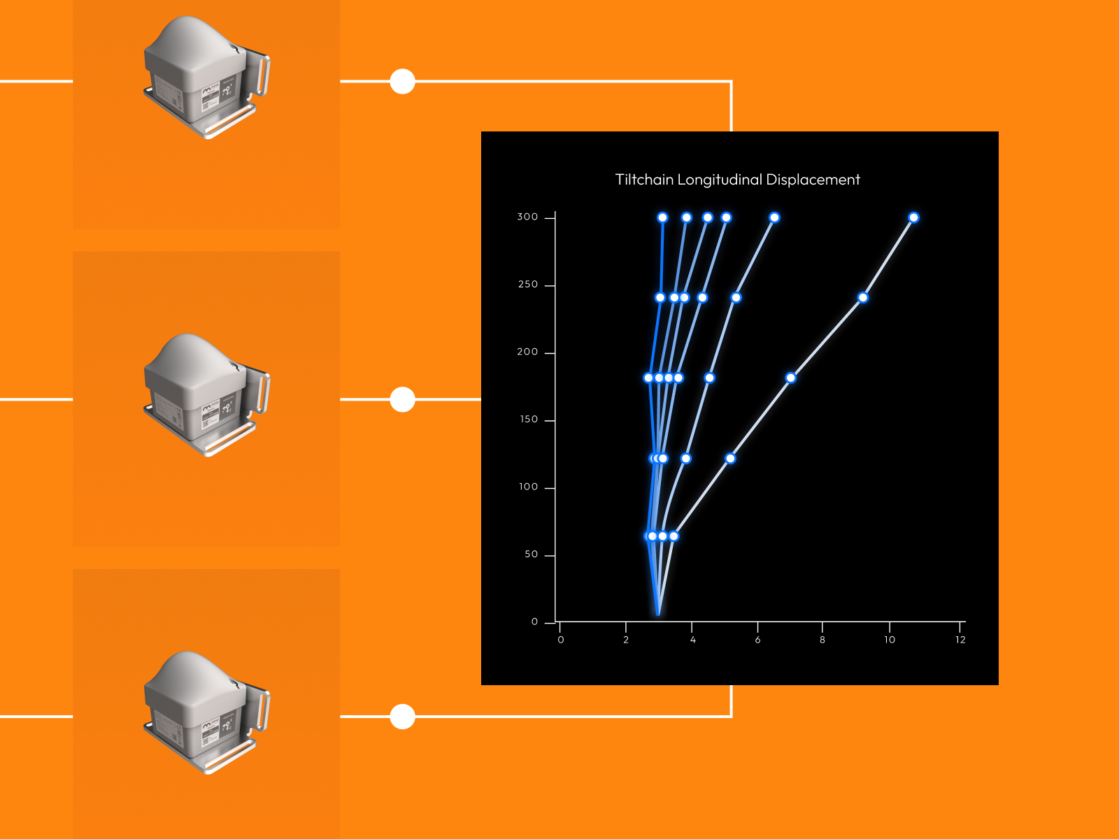
Building a chain

The next step for those monitoring extended structures is from the single inclinometer to the chain: multiple sensors in series, segment-by-segment integration, reconstruction of a deformation profile instead of a point rotation. The MyMove Tiltmeter Chain Tool applies the same angle-to-displacement conversion logic across the entire sensor chain, adding spatial integration segment by segment.

‍